【2】Kaggle 医学影像数据读取
赛题名称:RSNA 2024 Lumbar Spine Degenerative Classification
中文:腰椎退行性病变分类
kaggle官网赛题链接:https://www.kaggle.com/competitions/rsna-2024-lumbar-spine-degenerative-classification/overview
文章安排
①、如何用python读取dcm/dicom文件
②、基于matplotlib可视化
③、绘制频率分布直方图
④、代码汇总
文件依赖
# requirements.txt
# Python version 3.11.8
torch==2.3.1
torchvision==0.18.1
matplotlib==3.8.4
pydicom==2.4.4
numpy==1.26.4
pip install -r requirements.txt
读取dicom图像并做预处理
概述
本文中采取pydicom包读取dicom文件,其关键代码格式为:
dcm_tensor = pydicom.dcmread(dcm_file)
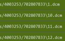
注意数据集的路径,其在train_images文件下存放了每一患者的数据,对于每一患者包含三张MRI图像,每张MRI图像存放为一个文件夹。
需要注意的是,MRI图像为三维图像(dicom格式),一般习惯性将其每个切片分别保存为一个dcm文件,因此一张dicom图像将被存为一个文件夹,如下图

我们可以采用如下路径访问该dicom文件:
"./train_images/4003253/702807833"
读取路径
为了读取dicom图像,我们需要写代码读取文件夹中的所有dcm文件
# dicom文件路径
dicom_dir = "./train_images/4003253/702807833"
# 保存所有dcm文件的路径
dicom_files = [os.path.join(dicom_dir, f) for f in os.listdir(dicom_dir) if f.endswith('.dcm')]
os.listdir:返回dicom_dir路径下的所有文件f.endswith('.dcm'):筛选所有dcm格式的文件os.path.join: 将dcm文件名添加到dicom_dir之后
示意:"./hello"+“1.dcm”->"./hello/1.dcm"
路径排序
这次的kaggle赛题所给的数据集中,文件名的迭代方式为:
1.dcm、2.dcm、...、9.dcm、10.dcm、11.dcm、...
这给我们带来了一定的麻烦,因为在os的文件名排序规则中,首先检索高位字母的ASCII码大小做排序,也就是说10.dcm将被认为是2.dcm前面的文件。
对此,本文采用正则表达式的方式,实现了依据文件名中数字大小排序。
def extract_number(filepath):
    # 获取文件名(包括扩展名)
    filename = os.path.basename(filepath)
    # 提取文件名中的数字部分,假设文件名以数字结尾,如 '1.dcm'
    match = re.search(r'(\d+)\.dcm$', filename)
    return int(match.group(1)) if match else float('inf')

# 基于数字句柄排序
dicom_files.sort(key=extract_number)
该代码效果如下:

读取图像
为读取dicom图像,我们需要依次读取每一个dcm文件,并将其最终打包为3D tensor,下述代码实现了该功能:
# 创建空列表保存所有dcm文件
dcm_list= []

# 迭代每一个文件
for dcm_file in dicom_files:
    # 读取文件
    dcm = pydicom.dcmread(dcm_file)
    # 将其转为numpy格式
    image_data = dcm.pixel_array.astype(np.float32)
    # 加入文件列表
    dcm_list.append(image_data)

# 将图片堆叠为3D张量
tensor_dcm = torch.stack([torch.tensor(image_data) for image_data in dcm_list])
数据预处理
常见的预处理方式有两种,归一化(Normalization)和量化(Quantization)
-
归一化:将数据缩放到某个标准范围内的过程。常见的归一化方法包括最小-最大归一化(Min-Max Normalization)和Z-score标准化(Z-score Normalization),前者将数据归一化至[0,1]范围,后者将数据转化为标准正态分布。本例中采用Min-Max方案。
-
量化:量化是将数据的值域退化到离散值的过程。常用于减少存储和计算成本,尤其在神经网络模型中。量化通常将浮点数值转换为整数值。量化前一般先进行归一化。
归一化的实现如下:
def norm_tensor(tensor_dicom):
    # 查找图像的最大值和最小值
    vmin, vmax = tensor_dicom.min(), tensor_dicom.max()
    # 归一化
    tensor_dicom= (tensor_dicom- vmax ) / (max_val - vmin)

    return tensor_dicom
实现基于method句柄选择预处理方式:
if method == "norm":
    # 归一化
    tensor_dcm = norm_tensor(tensor_dcm)
elif method == "uint8":
    # 归一化
    tensor_dcm = norm_tensor(tensor_dcm)
    # 量化
    tensor_dcm = (tensor_dcm * 255).clamp(0, 255).to(torch.uint8)
绘图
由于dicom图像为三维数据,可视化时我们一般将其在z轴上分为多个切片依次可视化,本文采用的方式是,采用5*5网格可视化至多25个切片。
def show_dciom(tensor_dicom):
    # 查找图像的最大最小值
    vmin, vmax = tensor_dicom.min(), tensor_dicom.max()

    # 创建一个图形窗口
    fig, axes = plt.subplots(5, 5, figsize=(15, 15))  # 5x5 网格布局

    count = 0
    length = tensor_dicom.size()[0]
    for i in range(25):
        if count < length:
            count += 1
        else:
            return
        # 获取当前图像的坐标
        ax = axes[i // 5, i % 5]
        # 显示图片
        ax.imshow(tensor_dicom[i], cmap='gray') # , vmin=vmin, vmax=vmax
        ax.axis('off')  # 关闭坐标轴

    plt.tight_layout() # 避免重叠
    plt.title(f"Layer {i}")
    plt.show()
这里有一点需要比较注意,在ax.imshow()函数中,我们指定了vmin和vmax参数;这是因为当该参数未被指定时,imshow函数将会自动调整点的亮度,使值最大的点对应255亮度,值最小的点对应0亮度。鉴于相邻切片最大、最小像素值可能存在较大差异,这将使得相邻切片的图像亮度较异常,如下图:

这两张图的左上角区域实际上亮度相近,但从可视化图像来看,存在较大差异,这将对观察带来误解。
可视化频率分布直方图
可视化MRI图像的频率分布直方图在医学影像处理中有重要意义,主要包括以下几个方面:
-
图像对比度分析:频率分布直方图可以显示MRI图像中不同灰度级别(或像素强度)的分布情况。通过分析直方图的形状和范围,可以了解图像的对比度。例如,直方图的分布范围较广表示图像对比度较高,能够更好地区分不同组织或结构。
-
图像均衡化:通过直方图均衡化,可以改善图像的对比度,使得低对比度的区域更加清晰。均衡化过程通过重新分配图像中的像素值,使得直方图的分布更加均匀,从而增强图像的视觉效果。
-
组织分割:频率分布直方图可以帮助确定适当的阈值,以进行图像分割。通过分析直方图,可以选择合适的阈值将不同组织或病变从背景中分离出来。
-
图像质量评估:直方图分析可以揭示图像的质量问题,例如过暗或过亮的图像,或者图像噪声的影响。通过直方图的形态,可以评估图像是否需要进一步的处理或优化。
在绘制频率分布直方图前,需要先将三维向量展平,本文采用plt.hist函数绘制
def show_hist(tensor_dicom):
    # 将所有图片的像素值展平为一个一维数组
    pixel_values = tensor_dicom.numpy().flatten()

    # 绘制直方图
    plt.figure(figsize=(10, 6))
    plt.hist(pixel_values, bins=50, color='gray', edgecolor='black')
    plt.title('Histogram of All Pixel Values')
    plt.xlabel('Pixel Value')
    plt.ylabel('Frequency')
    plt.grid(True)
    plt.show()
直方图呈现如下分步,在val=0附近有一高峰,这是因为MRI图像中大部分区域并不存在人体组织,为空值0。
倘若除零以外的点过分集中在较小值(<100),那么很可能是因为MRI图像中出现了一个亮度极大的噪点,使得以该噪点亮度为最值归一化质量较差,对于这种情形,可以用99%分位数代替最大值,并将99%分位数归一化至亮度为200. (比起归一化至255,这将允许亮度最大1%的像素点亮度值有区分)。
本例中图像质量均较高,故不需要做特殊处理。

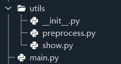
代码汇总
代码架构
主函数
# main.py
# Import custom utility functions
from utils import read_one_dicom, show_dciom, show_hist

# Define the directory containing the DICOM images
dicom_dir = "./train_images/4003253/1054713880"

# Read the DICOM image into a tensor with uint8 data type
tensor_dicom = read_one_dicom(dicom_dir, method="uint8")

# Display the DICOM image slices in a 5x5 grid layout
show_dciom(tensor_dicom)

# Plot the histogram of pixel values from the DICOM image slices
show_hist(tensor_dicom)

# Convert the tensor to a NumPy array for further processing or inspection
np_img = tensor_dicom.numpy()
包文件
from .preprocess import read_one_dicom

from .show import show_dciom
from .show import show_hist
读取&预处理
# preprocess.py
import numpy as np
import torch
import os
import re
import pydicom
from tqdm import tqdm

def norm_tensor(tensor_dicom):
    """
    Normalize the image tensor to the range [0, 1].

    Args:
        tensor_dicom (torch.Tensor): Tensor containing image data.

    Returns:
        torch.Tensor: Normalized image tensor.
    """
    # Calculate the maximum and minimum values of the image tensor
    vmin, vmax = tensor_dicom.min(), tensor_dicom.max()

    # Normalize the image tensor to the range [0, 1]
    tensor_dicom = (tensor_dicom - vmin) / (vmax - vmin)

    return tensor_dicom

def extract_number(filepath):
    """
    Extract the numeric part from the DICOM filename.

    Args:
        filepath (str): Path to the DICOM file.

    Returns:
        int: Extracted number from the filename. Returns float('inf') if not found.
    """
    # Get the filename (including extension)
    filename = os.path.basename(filepath)
    # Extract numeric part from filename, assuming filenames end with digits, e.g., '1.dcm'
    match = re.search(r'(\d+)\.dcm$', filename)
    return int(match.group(1)) if match else float('inf')

def read_one_dicom(dicom_dir, method = "", bar_title = ""):
    """
    Reads DICOM files from a directory and converts them into a PyTorch tensor.

    Args:
        dicom_dir (str): Directory containing DICOM files.
        method (str): Optional method to process the tensor ('norm' for normalization, 'uint8' for normalization and conversion to uint8).
        bar_title (str): Optional title for the progress bar.

    Returns:
        torch.Tensor: PyTorch tensor containing image data from DICOM files.
    """
    # Get all DICOM files and sort them based on numeric part of the filename
    dicom_files = [os.path.join(dicom_dir, f) for f in os.listdir(dicom_dir) if f.endswith('.dcm')]
    dicom_files.sort(key=extract_number)

    # Create an empty list to store image data
    dcm_list = []

    # Initialize tqdm progress bar
    with tqdm(total=len(dicom_files), desc='Processing DICOM files', unit='dcm', unit_scale=True, unit_divisor=1000000) as pbar:
        # Iterate over each DICOM file and read image data
        for count, dcm_file in enumerate(dicom_files, start=1):
            # Read the DICOM file
            dcm = pydicom.dcmread(dcm_file)

            # Extract and convert image data to a NumPy array
            image_data = dcm.pixel_array.astype(np.float32)

            # Add the image data to the list
            dcm_list.append(image_data)

            # Update progress bar description
            pbar.set_description(bar_title + 'Reading')

            # Update progress bar
            pbar.update(1)

    # Convert the list of image data to a PyTorch tensor and stack into a 3D tensor
    tensor_dicom = torch.stack([torch.tensor(image_data) for image_data in dcm_list])

    if method == "norm":
        # Normalize the image tensor
        tensor_dicom = norm_tensor(tensor_dicom)
    elif method == "uint8":
        # Normalize the image tensor
        tensor_dicom = norm_tensor(tensor_dicom)
        # Scale the tensor values to the range [0, 255] and convert to uint8 type
        tensor_dicom = (tensor_dicom * 255).clamp(0, 255).to(torch.uint8)

    return tensor_dicom
可视化、绘制直方图
# show.py
import numpy as np
import torch
import matplotlib.pyplot as plt

def show_dciom(tensor_dicom):
    """
    Display MRI image slices in a 5x5 grid layout.

    Parameters:
    tensor_dicom (torch.Tensor): Tensor containing MRI image slices, expected shape is (N, H, W),
                                 where N is the number of slices, and H and W are the height and width of the images.
    """
    # Calculate the minimum and maximum pixel values in the tensor
    vmin, vmax = tensor_dicom.min(), tensor_dicom.max()

    # Create a figure with a 5x5 grid layout
    fig, axes = plt.subplots(5, 5, figsize=(15, 15))  # 5x5 grid layout

    count = 0
    length = tensor_dicom.size(0)
    for i in range(25):
        if count < length:
            count += 1
        else:
            return
        # Get the current subplot's axis
        ax = axes[i // 5, i % 5]
        # Display the image
        ax.imshow(tensor_dicom[count - 1], cmap='gray', vmin=vmin, vmax=vmax)
        ax.axis('off')  # Hide the axis

    plt.tight_layout()  # Adjust layout to prevent overlap
    plt.title(f"Layer {i + 1}")  # Title indicating the last displayed slice
    plt.show()

def show_hist(tensor_dicom):
    """
    Plot the histogram of pixel values for all MRI image slices.

    Parameters:
    tensor_dicom (torch.Tensor): Tensor containing MRI image slices, expected shape is (N, H, W).
    """
    # Flatten all image pixel values into a single 1D array
    pixel_values = tensor_dicom.numpy().flatten()

    # Plot the histogram
    plt.figure(figsize=(10, 6))
    plt.hist(pixel_values, bins=50, color='gray', edgecolor='black')
    plt.title('Histogram of All Pixel Values')
    plt.xlabel('Pixel Value')
    plt.ylabel('Frequency')
    plt.grid(True)
    plt.show()
下篇预告
讨论本题的解题方法
制作不易,请帮我点一个免费的赞,谢谢!
本文来自博客园,作者:SXWisON,转载请注明原文链接:https://www.cnblogs.com/SXWisON/p/18370592